
1. Overview of Historical Volatility Indicator
1.1 What is Historical Volatility?
Historical Volatility (HV) is a statistical measure of the dispersion of returns for a given security or market index over a specific period. Essentially, it quantifies how much the price of an asset has varied in the past. This measure is expressed as a percentage and is often used by traders and investors to gauge the risk associated with a particular asset.
1.2 Importance in Financial Markets
The significance of Historical Volatility lies in its ability to provide insights into the past price movements of an asset, which is crucial for making informed trading decisions. High volatility indicates larger price swings and potentially higher risk, while low volatility suggests more stable and less risky price movements.
1.3 How Historical Volatility Differs from Implied Volatility
It’s important to distinguish Historical Volatility from Implied Volatility (IV). While HV looks at past price movements, IV is forward-looking and reflects the market’s expectations of future volatility, typically derived from options pricing. HV offers a factual record of past market behavior, whereas IV is speculative.
1.4 Applications in Trading and Investment
Traders often use Historical Volatility to assess whether an asset’s current price is high or low compared to its past fluctuations. This assessment can help in making decisions about entry and exit points in the market. Investors might use HV to adjust their portfolio’s risk exposure, preferring assets with lower volatility for a more conservative strategy.
1.5 Types of Historical Volatility
There are several types of Historical Volatility, including:
- Short-term Volatility: Typically calculated over periods like 10 or 20 days.
- Medium-term Volatility: Often measured over 50 to 60 days.
- Long-term Volatility: Analyzed over longer periods, such as 100 days or more.
Each type serves different trading strategies and investment horizons.
1.6 Advantages and Limitations
Advantages:
- Provides a clear historical perspective of market behavior.
- Useful for both short-term traders and long-term investors.
- Helps in identifying periods of high risk and potential market instabilities.
Limitations:
- Past performance is not always indicative of future results.
- Does not account for sudden market events or changes.
- May be less effective in markets with structural changes.
| Aspect | Description |
|---|---|
| Definition | Measure of the dispersion of returns for a security or market index over a specific period. |
| Expression | Presented as a percentage. |
| Usage | Assessing risk, understanding past price movements, trading strategy formulation. |
| Types | Short-term, Medium-term, Long-term. |
| Advantages | Historical perspective, utility across trading strategies, risk identification. |
| Limitations | Past performance limitation, sudden market event exclusion, structural change issues. |
2. Calculation Process of Historical Volatility
The calculation of Historical Volatility involves several steps, primarily revolving around statistical measures. The goal is to quantify the degree of variation in a security’s price over a specific period. Here is a breakdown of the process:
2.1 Data Collection
Firstly, collect the historical price data of the security or index. This data should include daily closing prices over the period for which you want to calculate volatility, typically 20, 50, or 100 trading days.
2.2 Calculating Daily Returns
Calculate the daily returns, which are the percentage change in price from one day to the next. The formula for daily return is:
Daily Return = [(Today's Closing Price / Yesterday's Closing Price) - 1] x 100
2.3 Standard Deviation Calculation
Next, calculate the standard deviation of these daily returns. The standard deviation is a measure of the amount of variation or dispersion in a set of values. A high standard deviation indicates greater volatility. Use the standard deviation formula applicable for your data set (sample or population).
2.4 Annualizing the Volatility
Since daily returns are used, the calculated volatility is daily. To annualize it (i.e., to convert it into an annual measure), multiply the standard deviation by the square root of the number of trading days in a year. The typical number used is 252, which is the average number of trading days in a year. Thus, the formula for annualized volatility is:
Annualized Volatility = Standard Deviation of Daily Returns x √252
| Step | Process |
|---|---|
| Data Collection | Gather historical daily closing prices |
| Daily Returns | Calculate the percentage change in price day-to-day |
| Standard Deviation | Compute the standard deviation of daily returns |
| Annualization | Multiply the standard deviation by √252 to annualize |
3. Optimal Values for Setup in Different Timeframes
3.1 Understanding Timeframe Selection
Selecting the optimal timeframe for the Historical Volatility (HV) Indicator is critical as it directly influences the interpretation and application of the indicator in various trading strategies. Different timeframes can provide insights into short-term, medium-term, and long-term volatility trends.
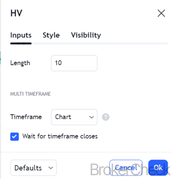
3.2 Short-Term Timeframes
- Duration: Typically ranges from 10 to 30 days.
- Application: Ideal for short-term traders like day traders or swing traders.
- Characteristic: Provides a quick, responsive measure of recent market volatility.
- Optimal Value: A shorter period, like 10 days, is often preferred for its sensitivity to recent market movements.
3.3 Medium-Term Timeframes
- Duration: Usually between 31 and 90 days.
- Application: Suited for traders with a medium-term outlook, such as position traders.
- Characteristic: Balances responsiveness with stability, offering a more rounded view of market volatility.
- Optimal Value: A 60-day period is a common choice, offering a balanced view of recent and slightly long-term trends.
3.4 Long-Term Timeframes
- Duration: Generally 91 days or more, often 120 to 200 days.
- Application: Useful for long-term investors focusing on broader market trends.
- Characteristic: Indicates the underlying trend in market volatility over an extended period.
- Optimal Value: A 120-day or 200-day period is frequently used, providing insight into longer-term market volatility dynamics.
3.5 Factors Influencing Optimal Timeframe Selection
- Trading Strategy: The chosen timeframe should align with the trader’s or investor’s strategy and goals.
- Market Conditions: Different market phases (bullish, bearish, sideways) may require adjustments in the chosen timeframe.
- Asset Characteristics: Volatility patterns can vary significantly across different assets, necessitating adjustments in the timeframe.
| Timeframe | Duration | Application | Characteristic | Optimal Value |
|---|---|---|---|---|
| Short-Term | 10-30 days | Day/Swing Trading | Responsive to recent market changes | 10 days |
| Medium-Term | 31-90 days | Position Trading | Balanced view of recent and past trends | 60 days |
| Long-Term | 91+ days | Long-term Investment | Reflects extended market volatility trends | 120 or 200 days |
4. Interpretation of Historical Volatility
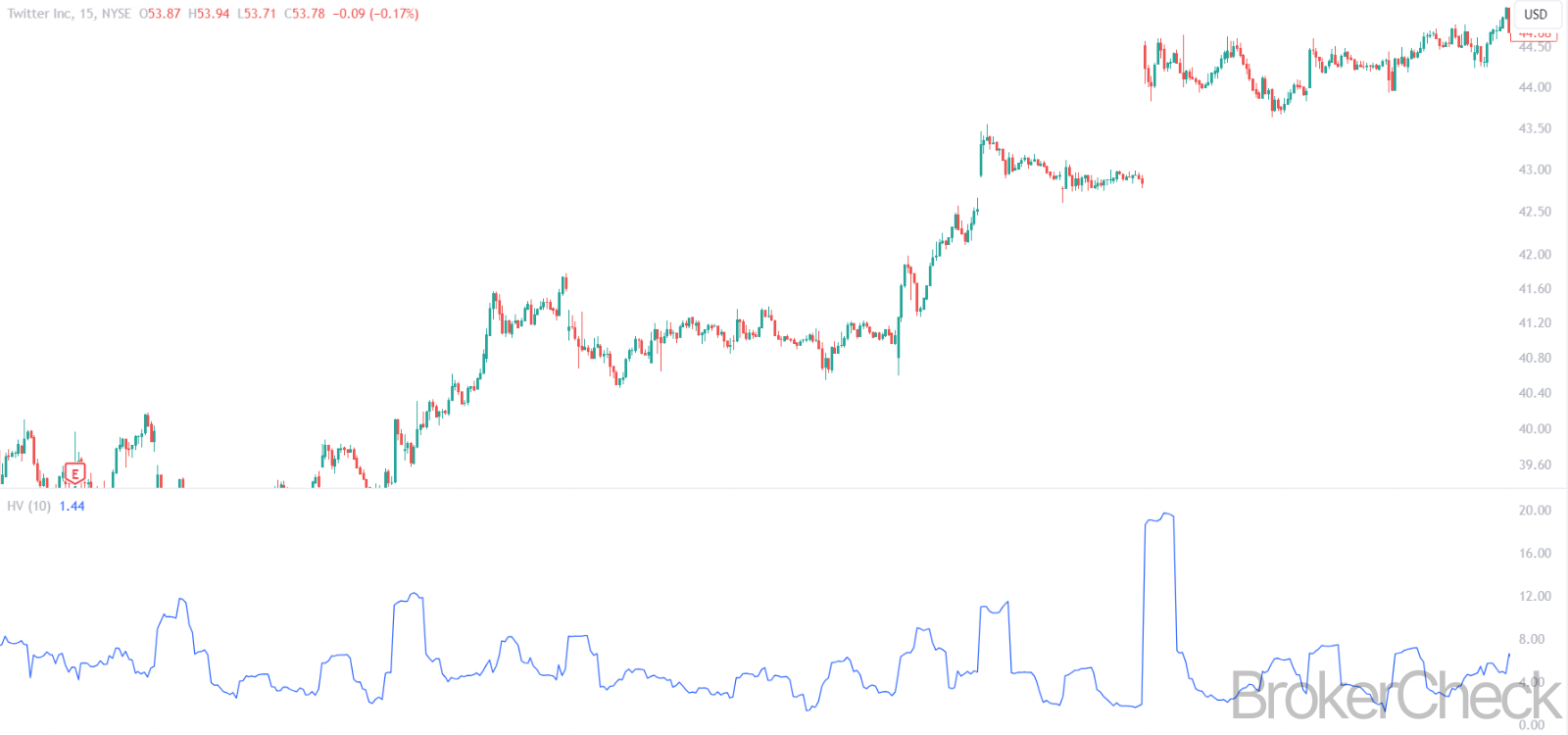
4.1 Understanding Historical Volatility Readings
Interpreting the Historical Volatility (HV) indicator involves analyzing its value to understand the volatility level of a security or market. Higher HV values indicate greater volatility, implying larger price swings, while lower values suggest less volatility and more stable price movements.
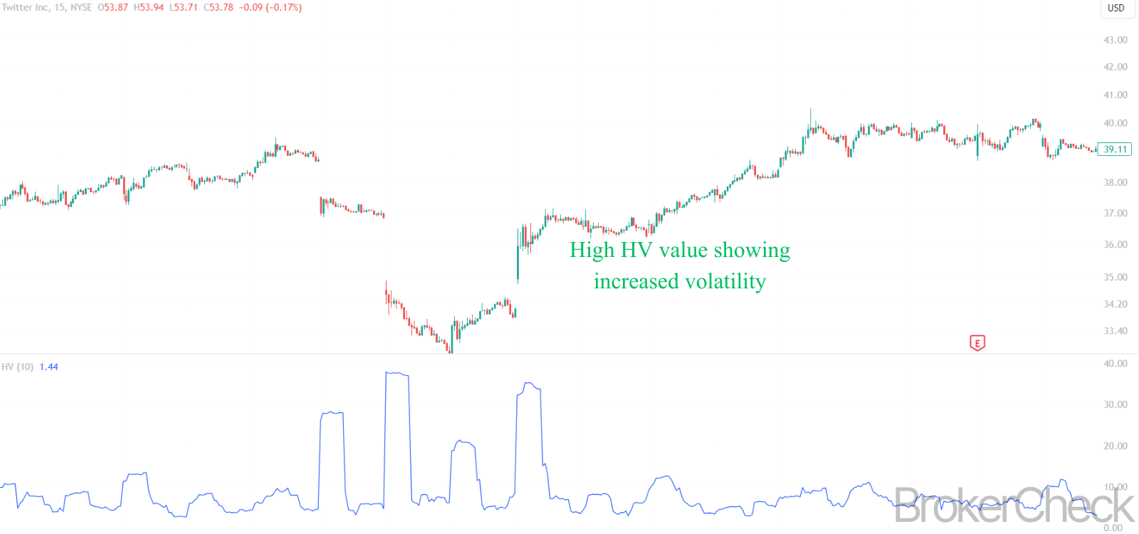
4.2 High Historical Volatility: Implications and Actions
- Meaning: High HV indicates that the price of the asset has been fluctuating significantly over the selected period.
- Implications: This can signal increased risk, potential market instability, or periods of market uncertainty.
- Investor Actions: Traders might look for short-term trading opportunities in such environments, while long-term investors may exercise caution or reconsider their risk management strategies.
4.3 Low Historical Volatility: Implications and Actions
- Meaning: Low HV suggests that the asset’s price has been relatively stable.
- Implications: This stability can indicate lower risk but may also precede periods of volatility (calm before the storm).
- Investor Actions: Investors may consider this an opportunity for longer-term investments, while traders might be wary of the potential for upcoming volatility spikes.
4.4 Analyzing Trends in Historical Volatility
- Rising Trend: A gradual increase in HV over time might indicate building market tension or impending significant price movements.
- Declining Trend: A decreasing HV trend can suggest market settling or a return to more stable conditions after a volatile period.
4.5 Using HV in the Market Context
Understanding the context is crucial. For instance, HV may rise during market events like earnings reports, geopolitical events, or economic announcements. It’s essential to correlate HV readings with market context for accurate interpretation.
| HV Reading | Implications | Investor Actions |
|---|---|---|
| High HV | Increased risk, potential instability | Short-term opportunities, risk reassessment |
| Low HV | Stability, possible upcoming volatility | Longer-term investments, caution for volatility spikes |
| Rising Trend | Building tension, impending movements | Prepare for potential market shifts |
| Declining Trend | Settling market, return to stability | Consider more stable market conditions |
5. Combining Historical Volatility with Other Indicators
5.1 The Synergy of Multiple Indicators
Integrating Historical Volatility (HV) with other technical indicators can enhance market analysis, providing a more holistic view. This combination helps in validating trading signals, managing risk, and identifying unique market opportunities.
5.2 HV and Moving Averages
- Combination Strategy: Pairing HV with Moving Averages (MAs) can be effective. For instance, a rising HV along with a moving average crossover can signal increasing market uncertainty coinciding with a potential trend change.
- Application: This combination is particularly useful in trend-following or reversal strategies.
5.3 HV and Bollinger Bands
- Combination Strategy: Bollinger Bands, which adjust themselves based on market volatility, can be used alongside HV to understand volatility dynamics better. For example, a high HV reading with a Bollinger Band expansion indicates heightened market volatility.
- Application: Ideal for spotting periods of high volatility which might result in breakout opportunities.

5.4 HV and Relative Strength Index (RSI)
- Combination Strategy: Using HV with the RSI can help in identifying whether a high volatility phase is associated with overbought or oversold conditions.
- Application: Useful in momentum trading, where traders can gauge the strength of the price movement along with volatility.
5.5 HV and MACD
- Combination Strategy: The Moving Average Convergence Divergence (MACD) indicator, when used with HV, assists in understanding whether volatile movements are backed by momentum.
- Application: Effective in trend-following strategies, especially in confirming the strength of trends.
5.6 Best Practices for Combining Indicators
- Complementary Analysis: Choose indicators that complement the HV to provide various analytical perspectives (trend, momentum, volume, etc.).
- Avoiding Overcomplication: Too many indicators can lead to analysis paralysis. Limit the number of indicators to maintain clarity.
- Backtesting: Always backtest strategies combining HV with other indicators to check their effectiveness in different market conditions.
| Combination | Strategy | Application |
|---|---|---|
| HV + Moving Averages | Signal validation for trend changes | Trend-following, reversal strategies |
| HV + Bollinger Bands | Identifying high volatility and breakouts | Breakout trading strategies |
| HV + RSI | Assessing volatility with market overbought/oversold conditions | Momentum trading |
| HV + MACD | Confirming trend strength alongside volatility | Trend-following strategies |
6. Risk Management with Historical Volatility
6.1 Role of HV in Risk Management
Historical Volatility (HV) is a crucial tool in risk management, providing insights into the past volatility of an asset. Understanding HV helps in tailoring risk management strategies according to the inherent volatility of the investment.
6.2 Setting Stop-Loss and Take-Profit Levels
- Application: HV can guide the setting of stop-loss and take-profit levels. Higher volatility may warrant wider stop-loss margins to avoid premature exits, while lower volatility could allow for tighter stops.
- Strategy: The key is to align stop-loss and take-profit levels with the volatility to balance risk and reward effectively.
6.3 Portfolio Diversification
- Assessment: HV readings across different assets can inform diversification strategies. A mix of assets with varying volatility levels can help in creating a balanced portfolio.
- Implementation: Incorporating assets with low HV can potentially stabilize the portfolio during turbulent market phases.
6.4 Position Sizing
- Strategy: Use HV to adjust position sizes. In higher volatility environments, reducing the position size can help manage risk, while in lower volatility settings, larger positions might be more feasible.
- Calculation: This involves assessing the asset’s HV in relation to the overall portfolio risk tolerance.
6.5 Market Entry and Exit Timing
- Analysis: HV can aid in determining optimal entry and exit points. Entering a trade during a period of low HV might precede a potential breakout, while exiting during high HV periods can be prudent to avoid large swings.
- Consideration: It’s important to combine HV analysis with other indicators for timing the market.
| Aspect | Application | Strategy |
|---|---|---|
| Stop-Loss/Take-Profit Levels | Adjusting margins based on HV | Align levels with asset volatility |
| Portfolio Diversification | Asset selection for balanced portfolio | Mix of high and low HV assets |
| Position Sizing | Manage exposure in volatile conditions | Adjust size based on asset’s HV |
| Market Timing | Identifying entry and exit points | Use HV for timing alongside other indicators |