


1. What is the Least Squares Moving Average?
The Least Squares Moving Average (LSMA), also known as the End Point Moving Average, is a type of moving average that applies the least squares regression method to the last n data points to determine the line of best fit. This line is then used to forecast the value at the next time point. Unlike traditional moving averages, the LSMA emphasizes the end of the data set, which is believed to be more relevant for predicting future trends.
The LSMA calculation involves finding the linear regression line that minimizes the sum of the squares of the vertical distances of the points from the line. This method is particularly effective in reducing the lag that is commonly associated with moving averages. By focusing on reducing the distance of the points from the line, the LSMA attempts to provide a more accurate and responsive indication of the direction and strength of a trend.
Traders often prefer the LSMA over other moving averages for its ability to closely track price movements and provide early signals of trend changes. It is especially useful in trending markets where the identification of the beginning and end of price trends is crucial for timely decision-making.
The adaptability of the LSMA allows it to be applied to various time frames, making it a versatile tool for traders who operate on different trading horizons, from intraday to long-term investment strategies. However, like all technical indicators, the LSMA should be used in conjunction with other tools and analysis methods to confirm signals and enhance trading accuracy.
2. How to Calculate the Least Squares Moving Average?
Calculating the Least Squares Moving Average (LSMA) requires several steps, involving statistical methods to fit a linear regression line to the closing prices of a security over a specified period. The formula for the linear regression line is:
y = mx + b
Where:
- y represents the predicted price,
- m is the slope of the line,
- x is the time variable,
- b is the y-intercept.
To determine the values for m and b, the following steps are taken:
- Assign sequential numbers to each period (e.g., 1, 2, 3, …, n) for the x values.
- Use the closing prices for each period as the y values.
- Calculate the slope (m) of the regression line using the formula:
m = (N Σ(xy) – Σx Σy) / (N Σ(x^2) – (Σx)^2)
Where:
- N is the number of periods,
- Σ denotes the summation over the periods in question,
- x and y are the individual period numbers and closing prices respectively.
- Compute the y-intercept (b) of the line with the formula:
b = (Σy – m Σx) / N
- Having determined m and b, you can forecast the next value by plugging in the corresponding x value (which would be N+1 for the next period) into the regression equation y = mx + b.
These calculations yield the end point of the LSMA at the current period, which can then be plotted as a continuous line over the price chart, moving forward as new data becomes available.
For practical application, most trading platforms include the LSMA as a built-in technical indicator, automating these calculations and updating the moving average in real-time. This convenience allows traders to focus on analyzing the market without the need for manual computation.
2.1. Understanding the Least Squares Moving Average Formula
Grasping the Slope and Intercept in LSMA
The LSMA formula’s core components, the slope (m) and y-intercept (b) are critical for understanding the trend’s trajectory. The slope reflects the rate at which the security’s price is changing over time. A positive slope indicates an uptrend, suggesting that prices are increasing as time progresses. Conversely, a negative slope points to a downtrend, with prices decreasing over the selected periods.
The y-intercept offers a snapshot of where the regression line crosses the y-axis. This intersection represents the predicted price when the time variable (x) is zero. In the context of trading, the y-intercept is less about its literal intersection point and more about its role in conjunction with the slope to calculate future prices.
Calculating Predictive Values with LSMA
Once the slope and y-intercept are determined, these values are applied to forecast future prices. The predictive nature of LSMA is encapsulated in the equation y = mx + b. Every new period’s value is estimated by inputting N+1 into the equation, where N is the number of the last known period. This predictive capability is what differentiates LSMA from simple moving averages, which merely average past prices without a directional component.
The LSMA’s focus on minimizing the sum of the squares of the vertical distances from the line effectively reduces the noise and produces a smoother representation of the price trend. This smoothing effect is particularly beneficial in volatile markets, where it can help traders discern the underlying trend amidst price fluctuations.
Practical Application of LSMA Values
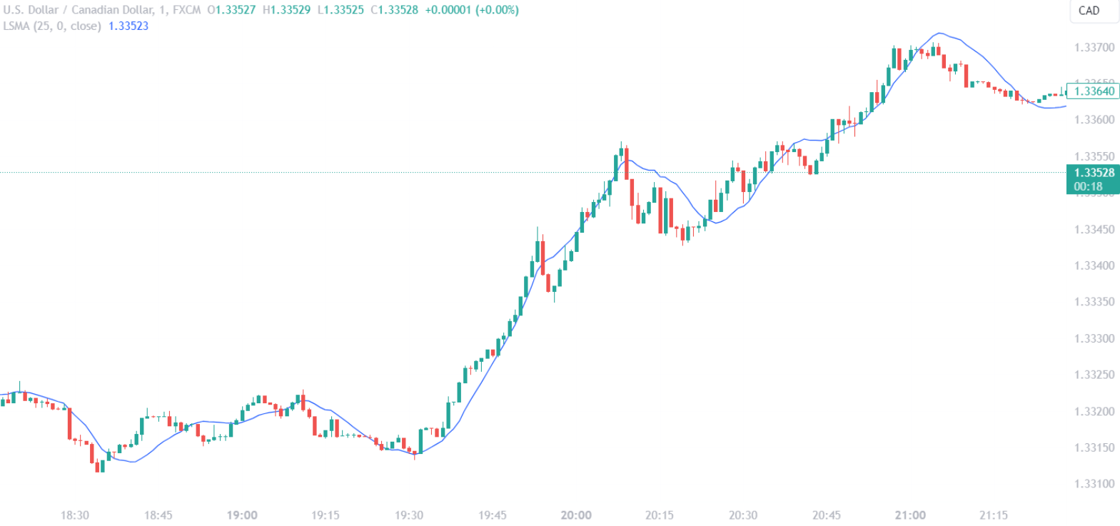
For traders, the practical application of LSMA values means monitoring the slope’s direction and magnitude. A steeper slope indicates a stronger trend, while a flattening slope suggests a potential weakening or reversal of the trend. Additionally, the LSMA line’s position relative to price action can serve as a signal: prices above the LSMA line may indicate bullish conditions, while prices below may suggest bearish conditions.
The LSMA formula’s ability to adapt to the latest market data makes it a dynamic and forward-looking tool. As new price data becomes available, the LSMA line is recalculated, ensuring that the moving average remains relevant and timely for decision-making.
| Component | Role in LSMA | Implication for Trading |
|---|---|---|
| Slope (m) | Rate of price change | Indicates trend direction and strength |
| Y-intercept (b) | Predicted price when x=0 | Used in formula to calculate future prices |
| Predictive Equation (y=mx+b) | Forecasts future prices | Helps anticipate trend continuations or reversals |
By understanding the mathematical underpinnings and practical implications of the LSMA formula, traders can better leverage this indicator in their market analysis and trading strategies.
2.2. Implementing Least Squares Moving Average in Python
Note: This method is for advanced Traders who know Python Programming. If it does not entrust youm you can skip to part 3.
To implement the Least Squares Moving Average (LSMA) in Python, one would typically employ libraries such as NumPy for numerical calculations and pandas for data manipulation. The implementation involves creating a function that takes a series of closing prices and the length of the moving average as inputs.
Firstly, a sequence of time values (x) is generated to match the closing prices (y). The NumPy library offers functions such as np.arange() to create this sequence, which is essential for calculating the summations required for the slope and intercept formulas.
NumPy also provides the np.polyfit() function, which offers a straightforward method to fit a least squares polynomial of a specified degree to the data. In the case of LSMA, a first-degree polynomial (linear fit) is appropriate. The np.polyfit() function returns the coefficients of the linear regression line, which corresponds to the slope (m) and y-intercept (b) in the LSMA formula.
import numpy as np
import pandas as pd

def calculate_lsma(prices, period):
    x = np.arange(period)
    y = prices[-period:]
    m, b = np.polyfit(x, y, 1)
    return m * (period - 1) + b
The above function can be applied to a pandas DataFrame containing the closing prices. By using the rolling method in combination with apply, the LSMA can be calculated for each window of the specified period throughout the dataset.
df['LSMA'] = df['Close'].rolling(window=period).apply(calculate_lsma, args=(period,))
In this implementation, the calculate_lsma function is designed to be used with the apply method, enabling the rolling computation of the LSMA values. The resultant LSMA column in the DataFrame provides a time series of the LSMA values that can be plotted against the closing prices to visualize the trend.
Integrating the LSMA into a Python trading script allows traders to automate trend analysis and potentially develop algorithmic trading strategies that respond to signals generated by the LSMA. As new price data is appended to the DataFrame, the LSMA can be recalculated, providing continuous trend analysis in real-time.
| Function | Use | Description |
|---|---|---|
np.arange() |
Generate sequence | Creates time values for the LSMA calculation |
np.polyfit() |
Fit regression line | Computes the slope and intercept for the LSMA |
rolling() |
Apply function over window | Enables rolling calculation of LSMA in pandas |
apply() |
Use custom function | Applies the LSMA calculation to each rolling window |
3. How to Configure Least Squares Moving Average Settings?
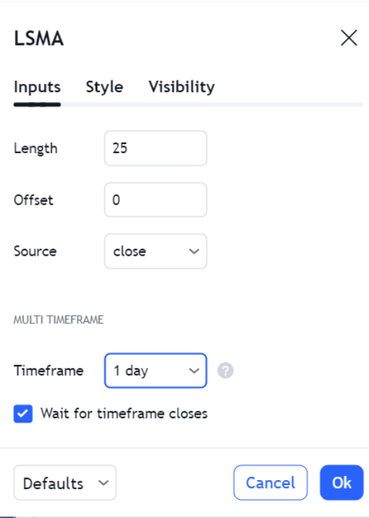
Configuring the Least Squares Moving Average (LSMA) settings accurately is pivotal to harnessing its full potential within a trading strategy. The primary configuration parameter for LSMA is the period length, which dictates the number of data points used in the regression analysis. This period can be fine-tuned based on the trader’s focus, whether it be short-term price movements or longer-term trend analysis. A shorter period length results in a more sensitive LSMA that reacts quickly to price changes, while a longer period provides a smoother line less prone to whipsaws.
Another critical setting is the source price. Although closing prices are commonly used, traders have the flexibility to apply the LSMA to open, high, low, or even an average of these prices. The choice of source price can affect the LSMA’s sensitivity and should align with the trader’s analytical approach.
To further refine the LSMA, traders might adjust the offset value, which shifts the LSMA line forward or backward on the chart. An offset can help align the LSMA more closely with the current price action or provide a clearer visual indication of the trend’s direction.
Advanced configurations may involve applying a multiplier to the slope or creating a channel around the LSMA by adding and subtracting a fixed value or a percentage from the LSMA line. These modifications can assist in identifying overbought and oversold conditions.
| Setting | Description | Impact |
|---|---|---|
| Period Length | Number of data points for regression | Influences sensitivity and smoothness |
| Source Price | Price type used (close, open, high, low) | Affects LSMA’s sensitivity to price |
| Offset | Shifts the LSMA line on the chart | Helps with visual alignment and trend indication |
| Multiplier/Channel | Adjusts slope or creates a range around LSMA | Assists in spotting market extremes |
Regardless of the settings chosen, it is crucial to backtest the LSMA with historical data to validate its effectiveness in the trading strategy. Continuous optimization may be necessary as market conditions evolve, ensuring that the LSMA settings remain congruent with the trader’s objectives and risk tolerance.
3.1. Determining the Optimal Period Length
Determining the Optimal Period Length for LSMA
The optimal period length for the Least Squares Moving Average (LSMA) is a function of trading style and market dynamics. Day traders may gravitate towards shorter periods, such as 5 to 20 days, to capture quick, significant movements. In contrast, swing traders or investors might consider periods ranging from 20 to 200 days to filter out market noise and align with longer-term trends.
Selecting the optimal period requires analyzing the trade-off between responsiveness and stability. A shorter period length increases responsiveness, providing early signals that can be crucial for capitalizing on short-term opportunities. However, this can also lead to false signals due to the LSMA’s heightened sensitivity to price spikes. On the other hand, a longer period length enhances stability, yielding fewer but potentially more reliable signals, suitable for confirming established trends.
Backtesting is indispensable for identifying the period length that aligns with historical performance. Traders should test various period lengths to ascertain the LSMA’s efficacy in generating profitable signals within the context of past market conditions. This empirical approach helps in gauging the indicator’s predictive power and adjusting the period length accordingly.
Volatility is another critical factor influencing period length. High-volatility environments may benefit from a longer period to avoid whipsaws, while lower-volatility conditions could be better suited to a shorter period, allowing traders to react swiftly to subtle price changes.
| Market Condition | Suggested Period Length | Rationale |
|---|---|---|
| High Volatility | Longer Period | Reduces noise and false signals |
| Low Volatility | Shorter Period | Increases sensitivity to price movements |
| Short-term Trading | 5-20 Days | Captures rapid market shifts |
| Long-term Trading | 20-200 Days | Filters out short-term fluctuations |
Ultimately, the optimal period length is not one-size-fits-all but rather a personalized parameter that requires fine-tuning to a trader’s specific risk profile, trading horizon, and the market’s volatility. Continuous evaluation and adjustment of the period length ensure that the LSMA remains a relevant and effective tool for market analysis.
3.2. Adjusting for Market Volatility
Volatility-Adjusted LSMA Periods
Adjusting the Least Squares Moving Average (LSMA) to account for market volatility involves calibrating the period length to reflect the prevailing market conditions. Volatility, a statistical measure of the dispersion of returns for a given security or market index, significantly impacts the behavior of moving averages. Highly volatile markets may render short-period LSMAs too erratic, generating excessive noise that can lead to misinterpretation of trend signals. Conversely, in low-volatility scenarios, a long-period LSMA may be too sluggish, failing to capture beneficial movements and trend shifts.
To mitigate these issues, traders can employ volatility indices, such as the VIX, to guide the adjustment of the LSMA period. A higher VIX reading, indicative of increased market volatility, might suggest extending the LSMA period to dampen the effects of price spikes and market noise. When the VIX is low, signaling calmer market conditions, a shorter LSMA period could be advantageous, allowing for a more agile response to price movements.
Incorporating a dynamic period adjustment mechanism based on volatility can further enhance the LSMA’s performance. This approach entails modifying the period length in real-time as volatility levels change. For instance, a simple volatility adjustment rule could increase the LSMA period by a percentage proportional to the rise in a volatility measure and vice versa.
Volatility bands can also be applied in conjunction with the LSMA to create a volatility-adjusted channel. The width of these bands fluctuates with changes in volatility, providing visual cues for potential breakout or consolidation phases. This method not only refines entry and exit signals but also aids in setting stop-loss levels that are congruent with current market volatility.
| Volatility Level | LSMA Adjustment | Purpose |
|---|---|---|
| High | Increase Period | Reduce noise and false signals |
| Low | Decrease Period | Enhance responsiveness to price changes |
Traders should note that while adjusting for volatility can improve the LSMA’s utility, it is not a panacea. Continuous monitoring and backtesting remain essential to ensure that the adjustments align with the overall trading strategy and risk management framework.
4. What are the Effective Least Squares Moving Average Strategies?
Trend Confirmation Strategy
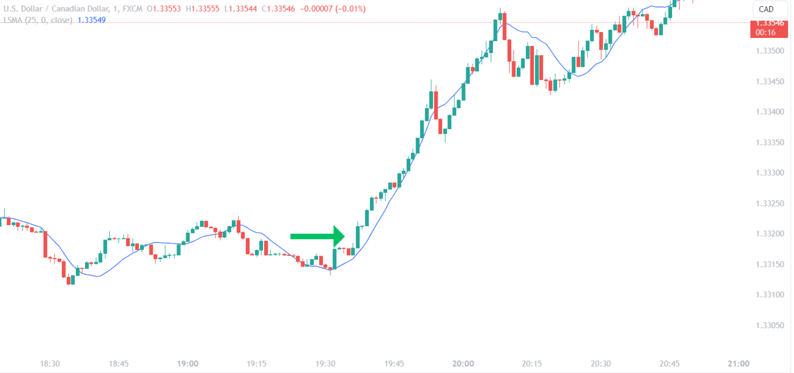
The Trend Confirmation Strategy uses the LSMA to validate the direction of the market trend. When the LSMA slope is positive and the price is above the LSMA line, traders may consider this a confirmation of an uptrend and an opportunity to open long positions. Conversely, a negative slope with price action below the LSMA could signal a downtrend, prompting traders to explore short positions. This strategy emphasizes the importance of slope direction and relative price position to make informed trading decisions.
Breakout Strategy
In the Breakout Strategy, traders watch for price movements that cross the LSMA line with significant momentum, which could indicate the beginning of a new trend. A breakout above the LSMA may be interpreted as a bullish signal, while a breakdown below the line could be seen as bearish. Traders often couple this strategy with volume analysis to confirm the strength of the breakout and to filter out false signals.
Moving Average Crossover Strategy
The Moving Average Crossover Strategy involves using two LSMAs of different periods. A common setup includes a short-period LSMA and a long-period LSMA. A crossover of the short-period LSMA above the long-period LSMA is typically treated as a buy signal, suggesting an emerging uptrend. Conversely, a crossover below may trigger a sell signal, indicating a potential downtrend. This dual LSMA approach allows traders to capture momentum shifts and can be particularly effective in trending markets.

Mean Reversion Strategy
Traders applying the Mean Reversion Strategy use the LSMA as a centerline to identify potential overextended price movements away from the trend. When prices deviate significantly from the LSMA and then begin to revert, traders might consider entering trades in the direction of the mean. This strategy is based on the premise that prices tend to return to the average over time, and the LSMA serves as a dynamic benchmark for mean reversion.
| Strategy | Description | Signal for Long Position | Signal for Short Position |
|---|---|---|---|
| Trend Confirmation | Validates trend direction using LSMA slope and price position | Positive slope with price above LSMA | Negative slope with price below LSMA |
| Breakout | Identifies new trends through LSMA line crossovers | Price breaks and holds above LSMA | Price breaks and holds below LSMA |
| Moving Average Crossover | Utilizes two LSMAs to spot momentum shifts | Short-period LSMA crosses above long-period LSMA | Short-period LSMA crosses below long-period LSMA |
| Mean Reversion | Capitalizes on price reversion to the LSMA | Price deviates from then reverts towards LSMA | Price deviates from then reverts towards LSMA |
These strategies represent a fraction of the potential applications of the LSMA in trading. Each strategy can be tailored to suit individual trading styles and market conditions. It’s crucial to conduct thorough backtesting and apply sound risk management practices when integrating these LSMA strategies into a trading plan.
4.1. Trend Following with LSMA
Trend Following with LSMA
In the realm of trend following, the Least Squares Moving Average (LSMA) serves as a potent indicator to gauge the direction and strength of market trends. Trend followers rely on the LSMA to identify sustainable price movements that could indicate a solid entry point. By observing the angle and direction of the LSMA, traders can ascertain the vigor of the current trend. A rising LSMA suggests upward momentum and, consequently, a potential to establish or maintain long positions. Conversely, a descending LSMA signals downward momentum, hinting at opportunities for short selling.
The LSMA’s efficiency in trend following is not solely tied to its direction but also its position in relation to the price. Price consistently remaining above a rising LSMA is an affirmation of bullish sentiment, while price persistently below a declining LSMA underscores bearish sentiment. Traders often look for these conditions to confirm their trend-following bias before executing trades.
Breakouts from consolidation phases into new trends are particularly significant when accompanied by the LSMA. A breakout with the LSMA moving in the same direction can reinforce the likelihood of a new trend forming. Traders can monitor the LSMA’s slope for acceleration or deceleration to judge the potential continuation or exhaustion of the trend.
| LSMA Behavior | Trend Implication | Potential Action |
|---|---|---|
| Rising LSMA | Upward Momentum | Consider Long Positions |
| Falling LSMA | Downward Momentum | Consider Short Positions |
| Price Above Rising LSMA | Bullish Trend Confirmation | Hold/Initiate Long Positions |
| Price Below Falling LSMA | Bearish Trend Confirmation | Hold/Initiate Short Positions |
Incorporating volume data can enhance trend following with the LSMA, as increased volume during trend confirmation can add conviction to the trade. Similarly, a divergence between volume and the LSMA slope may serve as a warning sign of a weakening trend.
Trend following with the LSMA is not a static strategy; it requires continuous monitoring of market conditions and the LSMA’s behavior. As the LSMA recalculates with each new data point, it reflects the latest price movements, allowing traders to stay aligned with the market’s current trajectory.
4.2. Mean Reversion and the LSMA
Mean Reversion and the LSMA
The concept of mean reversion suggests that prices and returns eventually move back towards the mean or average. This principle can be applied using the LSMA, which acts as a dynamic centerline representing the equilibrium level prices are expected to return to. Mean reversion strategies typically capitalize on extreme deviations from the LSMA, hypothesizing that prices will revert to this moving average over time.
For practical application, traders can establish thresholds for what constitutes an ‘extreme’ deviation. These thresholds can be set using standard deviation measurements or a percentage away from the LSMA. Trades are then initiated when the price crosses back over the threshold towards the LSMA, indicating the onset of mean reversion.
Setting Stop-Loss and Take-Profit Points is critical when employing mean reversion strategies with the LSMA. Stop-losses are typically placed beyond the established threshold to mitigate risk in the event of a continuation rather than a reversion. Take-profit points may be set near the LSMA, where the price is expected to stabilize.
| Threshold Type | Description | Application |
|---|---|---|
| Standard Deviation | Measures the amount of variation from the LSMA | Establishes boundaries for extreme price deviations |
| Percentage | Fixed percentage away from the LSMA | Defines overextended price conditions |
The LSMA’s dynamic nature makes it suitable for adapting to changing market conditions, which is beneficial in a mean reversion context. As the average price level shifts, the LSMA recalibrates, providing a continuously updated reference point for identifying mean reversion opportunities.
It’s important for traders to recognize that mean reversion strategies using the LSMA are not foolproof. Market conditions can change, and prices may not revert as expected. As such, risk management and backtesting are indispensable to validate the strategy’s effectiveness over different market cycles and conditions.
4.3. Combining LSMA with Other Technical Indicators
RSI and LSMA: Momentum Confirmation
Combining the Least Squares Moving Average (LSMA) with the Relative Strength Index (RSI) provides a multi-faceted view of market sentiment. The RSI, a momentum oscillator, measures the speed and change of price movements, typically on a scale of 0 to 100. An RSI value above 70 suggests an overbought condition, while below 30 indicates an oversold state. When the LSMA trend agrees with RSI signals, traders gain confidence in the prevailing momentum. For example, an RSI crossing above 70 coupled with an upward sloping LSMA may reinforce a bullish outlook.

MACD and LSMA: Trend Strength and Reversal
The Moving Average Convergence Divergence (MACD) is another powerful tool for use alongside the LSMA. The MACD measures the relationship between two moving averages of a security’s price. Traders look for the MACD line crossing above the signal line as a possible buy signal, and a cross below as a sell signal. When these MACD crossovers coincide with the LSMA indicating a trend in the same direction, it suggests a robust trend. Conversely, if the MACD diverges from the LSMA trend, it could signal a potential trend reversal.
Bollinger Bands and LSMA: Volatility and Trend Analysis
Bollinger Bands add a volatility dimension to the LSMA’s trend analysis. This indicator consists of a set of lines plotted two standard deviations (positively and negatively) away from a simple moving average (SMA) of the security’s price. When the LSMA resides within the Bollinger Bands, it confirms the trend within typical volatility boundaries. If the LSMA breaches the bands, it may indicate a volatility breakout and a stronger trend or a potential reversal if it occurs in the opposite direction of the prevailing trend.
Combining Technical Indicators with LSMA
| Indicator | Use with LSMA | Purpose |
|---|---|---|
| RSI | Confirm momentum | Validate overbought/oversold conditions with LSMA trend |
| MACD | Assess trend strength and potential reversals | Cross-validation of trend signals and divergences |
| Bollinger Bands | Gauge volatility and trend confirmation | Identify volatility breakouts and confirm trend strength within volatility norms |
Incorporating these indicators with the LSMA can yield a comprehensive trading approach, allowing for more nuanced analyses and potentially higher-probability trading setups. It is essential, however, to remember that no indicator is infallible. Each additional indicator introduces new parameters and potential for complexity, so traders must ensure a thorough understanding and testing of these combinations within their strategies.
5. What to Consider When Using Least Squares Moving Average in Trading?
Assessing Market Phase and LSMA Application
When employing the Least Squares Moving Average (LSMA), traders must first recognize the market phase—whether it’s trending or ranging—as the LSMA’s effectiveness varies accordingly. During trending phases, the LSMA can help identify and confirm the trend direction. However, in a ranging market, the LSMA may produce less reliable signals, as the average does not favor either direction strongly. Traders should complement the LSMA with other indicators suited for the current market phase to enhance decision-making accuracy.
LSMA Sensitivity and Data Noise
The sensitivity of the LSMA to recent price changes can be both an advantage and a drawback. Its responsiveness allows for early detection of trend shifts, but it may also react to short-term price spikes or drops, resulting in misleading signals. To mitigate this, traders should consider the overall price context and whether recent movements reflect a genuine trend change or simply temporary volatility.
Customization and Period Length
Customization of the LSMA period length is crucial, as there is no universal setting that suits all markets or trading styles. The chosen period should align with the trader’s strategy, with shorter periods for those seeking quick trades and longer periods for those looking to capture more significant trend movements. It’s imperative to backtest different period lengths to ensure the LSMA’s settings are optimized for the specific instrument and timeframe being traded.
Risk Management Integration
Integrating risk management into LSMA-based strategies cannot be overstated. The LSMA should not be the sole determinant of trade entries or exits. Instead, it should be part of a broader system that includes predefined risk parameters and stop-loss orders. The LSMA may help in setting dynamic stop-loss levels that adjust to the market’s current volatility and trend strength, but these should always be set within the bounds of the trader’s risk tolerance.
Continuous Learning and Adaptation
Lastly, traders should embrace continuous learning and adaptation when using the LSMA. As market conditions evolve, so should the application of the LSMA within a trading strategy. Regular review of the LSMA’s performance in light of recent market data can reveal necessary adjustments to its application, ensuring that the indicator remains a valuable tool in the trader’s arsenal.
| Consideration | Purpose |
|---|---|
| Market Phase Evaluation | Align LSMA use with trending or ranging markets |
| LSMA Sensitivity | Balance responsiveness with the potential for noise-induced signals |
| Customization and Backtesting | Optimize period lengths to match trading objectives and market behavior |
| Risk Management | Incorporate stop-loss orders and risk parameters to safeguard against false signals |
| Continuous Learning | Adapt LSMA usage to changing market conditions for sustained effectiveness |
5.1. Analyzing the Pros and Cons
Pros of the LSMA
The LSMA offers several advantages for traders. Its calculation method, which minimizes the sum of the squares of the deviations, typically provides a smoother line compared to traditional moving averages. This smoothness can help in identifying the underlying trend with less lag, giving traders the potential to catch trends earlier. Moreover, the LSMA’s adaptability to volatility adjustments allows for fine-tuning to different market conditions, increasing its utility in both high and low volatility environments.
| Advantage | Description |
|---|---|
| Smoothness | Reduces market noise and offers a clearer view of the trend. |
| Early Trend Identification | Minimizes lag in detecting trend changes, offering potential entry and exit signals sooner. |
| Volatility Adjustments | Customizable to market conditions, enhancing its responsiveness and accuracy. |
Cons of the LSMA
However, the LSMA is not without its drawbacks. Its sensitivity, while beneficial in trend detection, can also result in false signals during periods of market consolidation or when reacting to price spikes. Additionally, the LSMA does not provide much insight during ranging markets, as it may produce numerous crossovers with no clear direction. The need for extensive backtesting and customization for different timeframes and assets can also be time-consuming, potentially leading to over-optimization or curve-fitting issues.
| Disadvantage | Description |
|---|---|
| False Signals | Sensitivity to price changes may lead to misleading signals. |
| Ineffectiveness in Ranging Markets | Frequent crossovers without a clear trend can occur in sideways markets. |
| Need for Backtesting | Requires significant testing to tailor it to specific market conditions, which can be resource-intensive. |
In essence, while the LSMA can be a powerful tool in a trader’s arsenal, it should be used with a comprehensive understanding of its characteristics and in conjunction with other forms of analysis and risk management practices to mitigate its limitations.
5.2. Risk Management with LSMA
Dynamic Stop-Loss Placement
The LSMA’s ability to adapt to price movements makes it suitable for setting dynamic stop-loss levels. By placing a stop-loss order slightly below the LSMA for long positions, or above it for short positions, traders can align their risk management with the prevailing trend’s momentum. This method ensures that traders exit positions when the trend that prompted their entry may be reversing, thus protecting capital from larger drawdowns. The key is to set the stop-loss at a distance that accounts for the normal volatility of the asset to avoid being stopped out prematurely.
Position Sizing Based on Volatility
Traders can utilize the LSMA to inform position sizing by gauging the current market volatility. A more volatile market, suggested by wider swings around the LSMA, necessitates smaller position sizes to maintain a consistent risk level. Conversely, in less volatile conditions, traders might increase position sizes. This volatility-based approach ensures that the potential downside of each trade is proportionate to the overall trading capital, adhering to sound risk management principles.
| Market Condition | Position Sizing Strategy |
|---|---|
| High Volatility | Reduce position size to manage risk |
| Low Volatility | Consider increasing position size within risk tolerance |
Adjusting Risk Parameters
Adjusting risk parameters in response to changes in the LSMA slope can refine a trader’s risk management strategy. A steepening LSMA slope might indicate increasing trend strength, which could justify a tighter stop-loss to capture more profit. Conversely, a flattening slope might signal a weakening trend, prompting a wider stop-loss to avoid exiting on minor retractions. These adjustments should always be made within the context of the trader’s overall risk management framework and risk tolerance.
Integrating LSMA with Other Risk Indicators
While the LSMA can be central to setting dynamic stops and adjusting risk, integrating it with other risk indicators, such as the Average True Range (ATR), can provide a more holistic risk management approach. The ATR can help determine the stop-loss placement by providing a measure of the asset’s average volatility over a given period. Using the ATR in conjunction with the LSMA can help set more responsive stop-loss orders that are attuned to both the trend’s direction and the market’s volatility.
| Risk Indicator | Purpose in Risk Management |
|---|---|
| LSMA | Aligns stop-loss orders with trend direction and momentum |
| ATR | Informs stop-loss placement based on market volatility |
Continuous Risk Evaluation
The LSMA’s responsiveness to price changes necessitates continuous risk evaluation. As the indicator updates with each new data point, traders should reassess their stop-loss orders and position sizes to ensure they are still appropriate for the current market conditions. This evaluation should be a regular part of the trading routine, ensuring that risk management strategies remain effective as market dynamics evolve.
5.3. The Impact of Market Conditions on LSMA Performance
Market Volatility and LSMA Responsiveness
Market volatility significantly affects the LSMA’s performance. In highly volatile markets, the LSMA may exhibit greater fluctuations, which can lead to an increased number of false signals. Traders must be cautious, as these conditions can prompt the LSMA to react to price noise rather than true trend changes. Conversely, in markets exhibiting low volatility, the LSMA tends to provide more reliable signals, as its smoothing effect is more pronounced when price movements are less erratic.
Trend Strength and LSMA Signals
The strength of a trend is another critical factor impacting the LSMA’s effectiveness. Strong, sustained trends are conducive to the LSMA’s trend-following abilities, allowing for clearer and more actionable signals. When trends are weak or market conditions are choppy, the LSMA may produce ambiguous signals, making it challenging for traders to discern the trend’s direction confidently.
Market Phase and LSMA Utility
Understanding the market phase is essential when applying the LSMA. During trending phases, the LSMA’s utility is heightened as it can effectively track and confirm the trend’s direction. However, during range-bound phases, the LSMA’s performance falters, often resulting in a horizontal line that offers little to no actionable insight, potentially leading to multiple false entries and exits.
Adaptability and LSMA Customization
The LSMA’s adaptability to different market conditions is a double-edged sword. While it allows for customization to suit varying levels of volatility and different trend strengths, it also requires continual adjustment and optimization. Traders must be adept at fine-tuning the LSMA’s settings, such as the period length, to maintain its effectiveness across diverse market scenarios.
| Market Condition | LSMA Performance Impact | Trader’s Consideration |
|---|---|---|
| High Volatility | Increased false signals | Employ additional filters |
| Low Volatility | More reliable signals | Confidence in trend-following |
| Strong Trend | Clearer signals | Utilize LSMA for entries/exits |
| Weak/Choppy Trend | Ambiguous signals | Reduce reliance on LSMA |
| Trending Market | Enhanced utility | Align trades with LSMA direction |
| Ranging Market | Limited utility | Seek alternative indicators |
Traders must be agile in their approach, continuously assessing the prevailing market conditions to determine the LSMA’s current performance and potential impact on their trading decisions.