


1. Overview of Bollinger Bands %B Indicator
1.1 Introduction to Bollinger Bands %B
Bollinger Bands %B is a technical analysis tool invented by John Bollinger in the 1980s. It is derived from the original Bollinger Bands indicator, a widely-used tool in the trading community. The %B indicator provides a quantified measure of where the price is in relation to the bands, offering insights into the relative strength or weakness of a security.
1.2 Purpose of Bollinger Bands %B
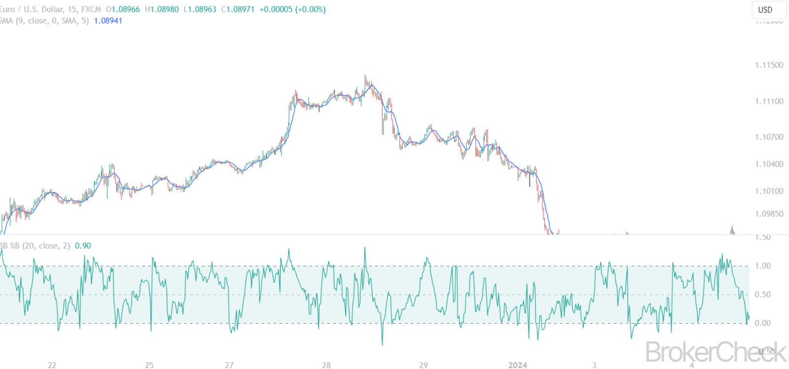
The primary purpose of Bollinger Bands %B is to identify overbought and oversold conditions in the market. It does this by comparing the current price of a security to the range defined by the Bollinger Bands. A value of 1 indicates that the price is at the upper band, 0 at the lower band, and 0.5 means the price is at the middle band (the moving average).
1.3 How It Differs from Traditional Bollinger Bands
While traditional Bollinger Bands focus on price volatility and relative price levels, Bollinger Bands %B zeroes in on the location of the price within the bands’ range. This provides a different perspective, focusing more on the relative position rather than the volatility aspect.
1.4 Common Uses in Trading
Traders commonly use Bollinger Bands %B for:
- Identifying overbought or oversold conditions.
- Confirming breakout signals when the price moves beyond the bands.
- Divergence trading, where discrepancies between the price trend and %B values indicate potential reversals.

1.5 Advantages and Limitations
Advantages:
- Versatility: Useful in various markets including stocks, forex, and commodities.
- Signal Clarity: Offers clear numerical values, making interpretation straightforward.
Limitations:
- Lagging Indicator: Like all indicators based on moving averages, it is inherently lagging.
- False Signals: Can generate false signals in highly volatile or trending markets.
| Aspect | Detail |
|---|---|
| Type of Indicator | Technical, derived from Bollinger Bands |
| Primary Use | Identifying overbought/oversold conditions |
| Calculation | Ratio of the difference between the price and lower band to the difference between the upper and lower bands |
| Typical Values | 0 (lower band), 0.5 (middle band), 1 (upper band) |
| Advantages | Versatility, clear numerical values |
| Limitations | Lagging nature, potential for false signals |
2. Calculation Process of Bollinger Bands %B
2.1 Understanding the Components
Before delving into the calculation, it’s crucial to understand the components involved in Bollinger Bands %B. This indicator is based on three main elements:
- Price: The current closing price of the security.
- Upper Bollinger Band: A moving average (typically 20 periods) plus a standard deviation (usually 2).
- Lower Bollinger Band: A moving average minus a standard deviation.
2.2 The Calculation Formula
The Bollinger Bands %B is calculated using the following formula:
%B = Current Price – Lower Band / Upper Band – Lower Band
This formula outputs a value between 0 and 1, indicating the relative position of the current price within the Bollinger Bands.
2.3 Step-by-Step Calculation
- Determine the Moving Average: Calculate the Simple Moving Average (SMA) for a specified number of periods (typically 20).
- Calculate the Standard Deviation: Find the standard deviation of the same number of periods used for the SMA.
- Form the Bands:
- Upper Band: SMA + (2 × standard deviation)
- Lower Band: SMA – (2 × standard deviation)
- Compute %B: Use the formula mentioned above to calculate the Bollinger Bands %B.
2.4 Example Calculation
Suppose the 20-period SMA of a stock is $100, and the standard deviation is $5. The upper band would be $110 ($100 + 2×$5), and the lower band would be $90 ($100 – 2×$5). If the current price is $102, then:
%B = {102 – 90}/{110 – 90} = {12}/{20} = 0.6
| Step | Component | Description |
|---|---|---|
| 1 | Moving Average | Typically a 20-period SMA |
| 2 | Standard Deviation | Based on the same period as the SMA |
| 3 | Upper/Lower Bands | SMA ± (2 × standard deviation) |
| 4 | %B Calculation | (Current Price – Lower Band) / (Upper Band – Lower Band) |
3. Optimal Values for Different Timeframes
3.1 Introduction to Timeframe Variability
The effectiveness of Bollinger Bands %B can vary significantly across different timeframes. Traders may need to adjust the settings to align with their trading strategy and the market’s characteristics. This section explores optimal parameter settings for various timeframes.
3.2 Short-Term Timeframes (Intraday to a Few Days)
For traders focusing on intraday to a few days, short-term fluctuations are critical.
Optimal Settings:
- Moving Average Period: 10 to 12 periods
- Standard Deviation Multiplier: 1.5 to 2
This setting increases sensitivity to price movements, suitable for capturing short-term trends and reversals.
3.3 Medium-Term Timeframes (Several Days to Weeks)
Medium-term traders balance the need for sensitivity with the avoidance of market noise.
Optimal Settings:
- Moving Average Period: 20 periods (standard)
- Standard Deviation Multiplier: 2 (standard)
These are the default settings, offering a balanced view of the market momentum and volatility.
3.4 Long-Term Timeframes (Months)
Long-term traders prioritize broader trends and smoother data over short-term fluctuations.
Optimal Settings:
- Moving Average Period: 50 to 60 periods
- Standard Deviation Multiplier: 2 to 2.5
Extended periods provide a more stable and less reactive indicator, suitable for long-term trend analysis.
3.5 Tailoring to Individual Trading Styles
It’s essential for traders to experiment with different settings to find what works best for their specific trading style and the assets they are trading. Market conditions and volatility can significantly impact the effectiveness of the Bollinger Bands %B indicator.

| Timeframe | Moving Average Period | Standard Deviation Multiplier | Suitability |
|---|---|---|---|
| Short-Term | 10-12 periods | 1.5-2 | High sensitivity for short-term trends |
| Medium-Term | 20 periods (standard) | 2 (standard) | Balanced for moderate-term analysis |
| Long-Term | 50-60 periods | 2-2.5 | Stable for long-term trend following |
4. Interpretation of Bollinger Bands %B Readings
4.1 Understanding %B Values
The interpretation of Bollinger Bands %B is crucial for making informed trading decisions. The %B value indicates a security’s position relative to the upper and lower bands, offering insights into market conditions.
4.2 Interpreting Specific %B Values
- %B Above 1.0: This suggests the price is above the upper band, indicating an overbought market condition. Traders often view this as a sell signal or a warning of a potential price reversal.
- %B Below 0.0: Conversely, a %B value below 0.0 means the price is below the lower band, signaling an oversold condition. This is often considered a buy signal or an indication of a potential upward reversal.
- %B Around 0.5: A %B value near 0.5 implies that the price is at the middle band (the moving average), suggesting a neutral market condition.

4.3 Using %B for Confirmation
The %B indicator is often used in conjunction with other technical analysis tools for confirmation:
- Confirming Trend Reversals: A reversal in %B direction can confirm potential trend reversals identified by other indicators.
- Validating Breakouts: A sustained move of %B above 1.0 or below 0.0 can validate a price breakout beyond the Bollinger Bands.
4.4 Divergence Analysis
Divergence occurs when the price movement and the %B value move in opposite directions. This can be a powerful signal for potential reversals:
- Bullish Divergence: When the price hits new lows, but %B forms higher lows.
- Bearish Divergence: When the price reaches new highs, but %B forms lower highs.
| %B Value | Market Implication | Potential Action |
|---|---|---|
| Above 1.0 | Overbought condition | Possible sell signal |
| Below 0.0 | Oversold condition | Possible buy signal |
| Around 0.5 | Neutral market condition | Neutral stance |
| Divergence | Potential reversal | Monitor for trend changes |
5. Combining Bollinger Bands %B with Other Indicators
5.1 Synergy in Technical Analysis
Combining Bollinger Bands %B with other technical indicators can enhance analysis, provide more robust signals, and reduce false positives. This multi-indicator approach can offer a more comprehensive view of market conditions.
5.2 Bollinger Bands %B and Moving Averages
- Strategy: Utilize Bollinger Bands %B in conjunction with simple or exponential moving averages (SMA/EMA).
- Purpose: To identify trend strength and potential reversal points.
- Application: A rising moving average with a high %B value can confirm an uptrend, while a falling moving average with a low %B value might confirm a downtrend.
5.3 Combining with Relative Strength Index (RSI)
- Strategy: Pair Bollinger Bands %B with the Relative Strength Index (RSI).
- Purpose: To identify overbought or oversold conditions more accurately.
- Application: An RSI reading above 70 and a high %B value can signal an overbought condition, whereas an RSI below 30 with a low %B value can indicate an oversold condition.
5.4 Using with Stochastic Oscillator
- Strategy: Combine Bollinger Bands %B with the Stochastic Oscillator.
- Purpose: For confirmation of momentum and potential reversal points.
- Application: Look for situations where both the Stochastic Oscillator and %B are indicating overbought or oversold conditions for stronger signals.
5.5 Integration with Volume Indicators
- Strategy: Use Bollinger Bands %B alongside volume indicators like On-Balance Volume (OBV).
- Purpose: To confirm breakout signals and the strength of trends.
- Application: An increase in volume coupled with a %B value exceeding 1.0 can confirm a bullish breakout, and vice versa for bearish breakouts.
| Combined Indicator | Purpose | Application |
|---|---|---|
| Moving Averages (SMA/EMA) | Trend identification | Confirm uptrend/downtrend |
| Relative Strength Index (RSI) | Overbought/Oversold conditions | Confirm overbought/oversold signals |
| Stochastic Oscillator | Momentum and reversals | Confirm momentum direction |
| Volume Indicators (e.g., OBV) | Confirm breakouts and trend strength | Validate strength of breakouts |
6. Risk Management with Bollinger Bands %B
6.1 Importance of Risk Management in Trading
Incorporating risk management strategies is essential when using technical indicators like Bollinger Bands %B. Effective risk management helps in protecting capital and optimizing trading performance.
6.2 Setting Stop-Loss Orders
- Strategy: Utilize %B readings to set stop-loss orders.
- Application: Place stop-loss orders at a level where the %B indicates a reversal of the current trend. For example, in a long position, set a stop-loss where the %B dips below a certain threshold, signaling a potential downtrend.
6.3 Position Sizing Based on Volatility
- Strategy: Adjust position sizes based on the width of the Bollinger Bands.
- Application: In periods of high volatility (wider bands), reduce position size to manage risk. Conversely, in lower volatility (narrower bands), consider increasing position size, as price movements are expected to be smaller.
6.4 Diversifying with Multiple Indicators
- Strategy: Combine Bollinger Bands %B with other indicators for diversified risk management.
- Application: Use additional indicators to confirm %B signals. This helps avoid relying solely on one indicator, reducing the risk of false signals.
6.5 Implementing Profit Targets
- Strategy: Use %B readings to set realistic profit targets.
- Application: Establish profit targets at levels where the %B suggests a weakening of the current trend. For instance, in a long position, set a profit target where the %B nears 1.0, indicating a potential overbought condition.
| Risk Management Strategy | Application | Purpose |
|---|---|---|
| Setting Stop-Loss Orders | Based on %B reversal signals | To limit potential losses |
| Position Sizing | Adjusted according to Bollinger Bands width | To manage risk during different volatility levels |
| Diversifying with Multiple Indicators | Combining %B with other technical tools | To reduce reliance on a single indicator |
| Implementing Profit Targets | Setting targets based on %B levels | To lock in profits at optimal points |